Data Cleaning

This page shows the raw data, the code used to clean it, and the modified data. It’s a journal of my data cleaning process. Please be aware that this page contains both Python and R code, thus you should avoid running the source code all at once.

ncaahoopR

2021-22 Season

Let’s clean the Villanova 2021-22 data with R:

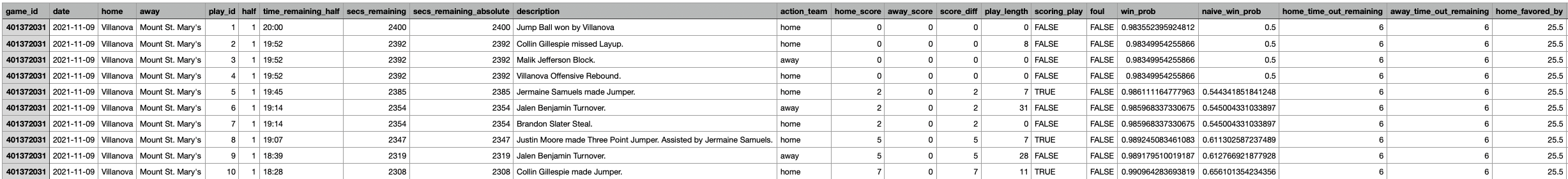
Here is a screen shot of the first few rows and columns of the raw data:

library(tidyverse)

After we load in relevant libraries, we can read in the data and check its shape.

nova2122 <- read.csv('./data/raw_data/villanova2122.csv')

dim(nova2122)

1. 11405
2. 39

What columns does the NCAA data have?

# what are the column names?
colnames(nova2122)

1. 'game_id'
2. 'date'
3. 'home'
4. 'away'
5. 'play_id'
6. 'half'
7. 'time_remaining_half'
8. 'secs_remaining'
9. 'secs_remaining_absolute'
10. 'description'
11. 'action_team'
12. 'home_score'
13. 'away_score'
14. 'score_diff'
15. 'play_length'
16. 'scoring_play'
17. 'foul'
18. 'win_prob'
19. 'naive_win_prob'
20. 'home_time_out_remaining'
21. 'away_time_out_remaining'
22. 'home_favored_by'
23. 'total_line'
24. 'referees'
25. 'arena_location'
26. 'arena'
27. 'capacity'
28. 'attendance'
29. 'shot_x'
30. 'shot_y'
31. 'shot_team'
32. 'shot_outcome'
33. 'shooter'
34. 'assist'
35. 'three_pt'
36. 'free_throw'
37. 'possession_before'
38. 'possession_after'
39. 'wrong_time'

The dataset appears fairly clean; however, to focus specifically on shooting data, we’ll exclude rows without a designated shooter (e.g., turnovers, steals, rebounds, or blocks) where the shooter is marked as NA. After this refinement, we’ll reassess the shape of the data.

nova2122 <- nova2122 %>%
  filter(!is.na(shooter))

# let's check the shape of the data
dim(nova2122)

1. 5399
2. 39

We can see that about 5,000 rows were removed and we are left with a little over half of the initial data. In the below chunk, we create a new column, “shooter_team,” based on the action team. We create another column “shot_sequence” that tracks consecutive made or missed shots by a shooter in each game half, and then use that column to create a “previous_shots” column that indicates the number of consecutive shots (made or missed) by the shooter before the current shot. This modified dataset is then saved as a CSV file.

# only taking the columns I want from this dataset
sample <- nova2122 %>% select(game_id, play_id, half, shooter, shot_outcome, home, away, action_team)

#creating a new column shooter_team
sample <- sample %>%
  mutate(
    shooter_team = ifelse(action_team == "home", home, away))

# Specifying columns to drop and removing them from the dataframe
columns_to_drop <- c("home", "away", "action_team")

sample <- sample %>%
  select(-one_of(columns_to_drop))

#I want to create a previous_shots column that says how many shots the shooter has made or missed in a row before the current shot they are taking
sample <- sample %>%
  mutate(
    shot_outcome_numeric = ifelse(shot_outcome == "made", 1, -1)
  )

sample <- sample %>%
  group_by(game_id, half, shooter) %>%
  arrange(play_id) %>%
  mutate(
    shot_sequence = cumsum(shot_outcome_numeric)) %>%
  ungroup()

sample3 <- sample %>%
  mutate(
    shot_sequence = ifelse(shot_outcome == "made" & shot_sequence <= 0, 1,
                  ifelse(shot_outcome == "missed" & shot_sequence >= 0, -1, shot_sequence))
  )

sample3 <- sample3 %>%
  group_by(game_id, half, shooter) %>%
  arrange(play_id) %>%
  mutate(
    previous_shots = ifelse(row_number() == 1, 0, lag(shot_sequence, default = 0))
  ) %>%
  ungroup()

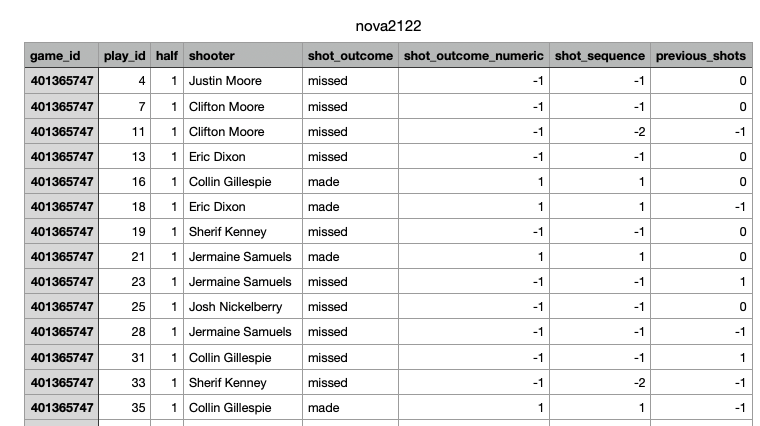
write.csv(sample3, file = "./data/modified_data/nova2122.csv", row.names = FALSE)

Here is a screen shot of the modified data:

2019-20 Season

We can replicate the process for the 2019-20 NCAA data. The following code mirrors the one used above but is tailored to the 2019-20 season.

# let's load in the data
nova1920 <- read.csv('./data/raw_data/villanova1920.csv')

# let's check the shape of the data
dim(nova1920)

1. 9581
2. 39

# what are the column names?
colnames(nova1920)

1. 'game_id'
2. 'date'
3. 'home'
4. 'away'
5. 'play_id'
6. 'half'
7. 'time_remaining_half'
8. 'secs_remaining'
9. 'secs_remaining_absolute'
10. 'description'
11. 'action_team'
12. 'home_score'
13. 'away_score'
14. 'score_diff'
15. 'play_length'
16. 'scoring_play'
17. 'foul'
18. 'win_prob'
19. 'naive_win_prob'
20. 'home_time_out_remaining'
21. 'away_time_out_remaining'
22. 'home_favored_by'
23. 'total_line'
24. 'referees'
25. 'arena_location'
26. 'arena'
27. 'capacity'
28. 'attendance'
29. 'shot_x'
30. 'shot_y'
31. 'shot_team'
32. 'shot_outcome'
33. 'shooter'
34. 'assist'
35. 'three_pt'
36. 'free_throw'
37. 'possession_before'
38. 'possession_after'
39. 'wrong_time'

# this data looks relatively clean, but we want only shooting data
# let's get rid of rows where there isn't a shooter
# this would be rows where the shooter is NA
# such as a turnover, steal, rebound, or block
nova1920 <- nova1920 %>%
  filter(!is.na(shooter))

# let's check the shape of the data
dim(nova1920)

1. 4543
2. 39

# we can see that we removed about 5,000 rows and are left with just a little over half the initial data

# only taking the columns I want from this dataset
sample <- nova1920 %>% select(game_id, play_id, half, shooter, shot_outcome, home, away, action_team)

#creating a new column shooter_team
sample <- sample %>%
  mutate(
    shooter_team = ifelse(action_team == "home", home, away))

# Specifying columns to drop and removing them from the dataframe
columns_to_drop <- c("home", "away", "action_team")

sample <- sample %>%
  select(-one_of(columns_to_drop))

#I want to create a previous_shots column that says how many shots the shooter has made or missed in a row before the current shot they are taking
sample <- sample %>%
  mutate(
    shot_outcome_numeric = ifelse(shot_outcome == "made", 1, -1)
  )

sample <- sample %>%
  group_by(game_id, half, shooter) %>%
  arrange(play_id) %>%
  mutate(
    shot_sequence = cumsum(shot_outcome_numeric)) %>%
  ungroup()

sample3 <- sample %>%
  mutate(
    shot_sequence = ifelse(shot_outcome == "made" & shot_sequence <= 0, 1,
                  ifelse(shot_outcome == "missed" & shot_sequence >= 0, -1, shot_sequence))
  )

sample3 <- sample3 %>%
  group_by(game_id, half, shooter) %>%
  arrange(play_id) %>%
  mutate(
    previous_shots = ifelse(row_number() == 1, 0, lag(shot_sequence, default = 0))
  ) %>%
  ungroup()

write.csv(sample3, file = "./data/modified_data/nova1920.csv", row.names = FALSE)

News API

Let’s clean this textual data using python:

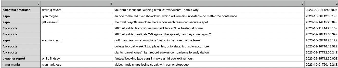
Here is a picture of the first few rows of the raw data:

import pandas as pd
import numpy as np
from sklearn.feature_extraction.text import CountVectorizer

This code reads sentiment scores from a JSON file, extracts titles and descriptions, assigns sentiment labels based on compound scores, forms a DataFrame, and saves the output, including titles, to a CSV file.

# Load the sentiment scores from the JSON file
with open('sentiment_scores.json', 'r') as json_file:
    sentiment_scores = json.load(json_file)

# Create lists to store data
titles = []  # List to store document titles
descriptions = []   # List to store document descriptions
sentiment_labels = []  # List to store sentiment labels

# Extract the scores, titles, descriptions, and labels
for idx, item in enumerate(sentiment_scores, start=1):
    titles.append(item.get('title', ''))  # Get the title of the document
    descriptions.append(item.get('description', ''))    # Get the description of the document
    sentiment_score = item.get('sentiment_score', {})
    
    # Determine the sentiment label based on the compound score
    if sentiment_score.get('compound', 0) > 0:
        sentiment_labels.append('positive')
    elif sentiment_score.get('compound', 0) == 0:
        sentiment_labels.append('neutral')
    else:
        sentiment_labels.append('negative')

# Create a DataFrame
data = {
    'Title': titles,
    'Description': descriptions,
    'Sentiment Label': sentiment_labels
}

df_with_labels = pd.DataFrame(data)

# Save to CSV
df_with_labels.to_csv('./data/modified_data/sentiment_scores_with_titles.csv', index=False)

Individual Player Data

Let’s clean the Aaron Judge game data with python:

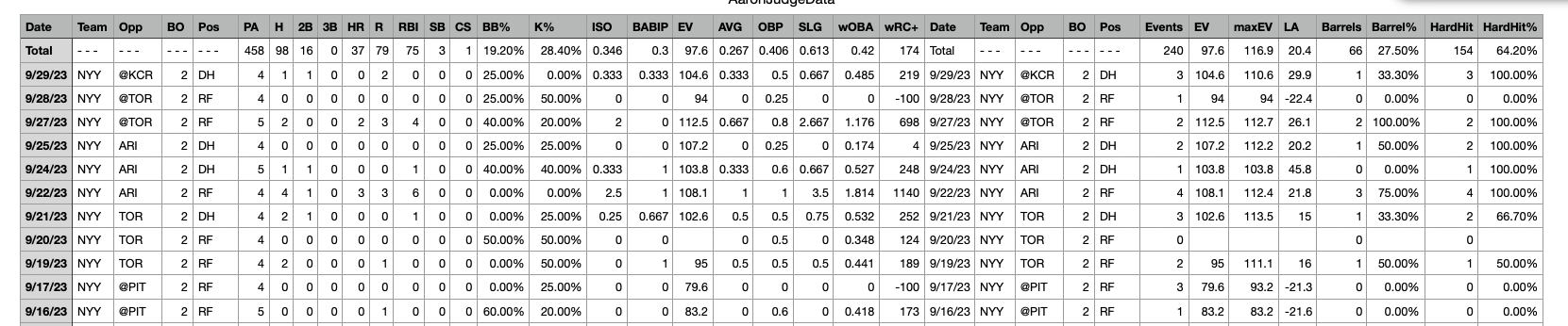
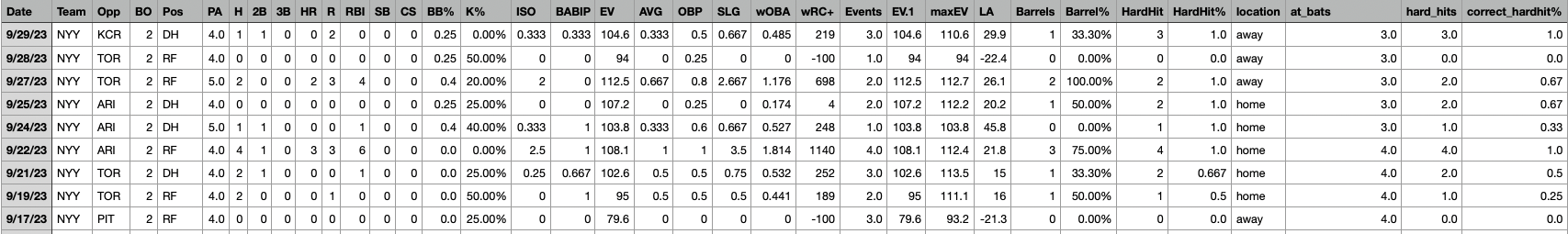
Here is a screen shot of the first few rows of the raw data:

After loading in relevant libraries and reading in the data, let’s check the shape of the dataset.

import pandas as pd
import numpy as np

#reading in the file
aaronjudge = pd.read_csv('./data/raw_data/AaronJudgeData.csv')

#how many rows are in this dataset?
aaronjudge.shape

(111, 37)

What are the column names?

#what are the column names?
aaronjudge.columns

Index(['Date', 'Team', 'Opp', 'BO', 'Pos', 'PA', 'H', '2B', '3B', 'HR', 'R',
       'RBI', 'SB', 'CS', 'BB%', 'K%', 'ISO', 'BABIP', 'EV', 'AVG', 'OBP',
       'SLG', 'wOBA', 'wRC+', 'Date.1', 'Team.1', 'Opp.1', 'BO.1', 'Pos.1',
       'Events', 'EV.1', 'maxEV', 'LA', 'Barrels', 'Barrel%', 'HardHit',
       'HardHit%'],
      dtype='object')

Let’s remove repeated columns and check the column names again.

#removing the repeated columns
columns_to_remove = ['Date.1', 'Team.1', 'Opp.1', 'BO.1', 'Pos.1']
aaronjudge.drop(columns=columns_to_remove, inplace=True)
aaronjudge.columns

Index(['Date', 'Team', 'Opp', 'BO', 'Pos', 'PA', 'H', '2B', '3B', 'HR', 'R',
       'RBI', 'SB', 'CS', 'BB%', 'K%', 'ISO', 'BABIP', 'EV', 'AVG', 'OBP',
       'SLG', 'wOBA', 'wRC+', 'Events', 'EV.1', 'maxEV', 'LA', 'Barrels',
       'Barrel%', 'HardHit', 'HardHit%'],
      dtype='object')

I believe that the intiial row with the column names is repeated throughout the data, let’s check if that is indeed the case.

# i belive the initial row with the column names is repeated throughou the data. let's check
print((aaronjudge['Date'] == 'Date').sum())

5

Let’s remove these rows and check the shape again.

# let's remove these rows and then check the shape again
aaronjudge.drop(aaronjudge[aaronjudge['Date'] == 'Date'].index, inplace=True)
aaronjudge.shape

(106, 32)

There is a total row at the bottom of the data, let’s remove that as well.

# there is also a total row which I want to remove as well. let's do that now
aaronjudge.drop(aaronjudge[aaronjudge['Date'] == 'Total'].index, inplace=True)
aaronjudge.shape

(105, 32)

So far, I have removed 6 rows and 5 columns. I want to create a location column (home or away) based on the “@” in the “Opp” column. Let’s do that now and check the values of the new column.

# so far, I have removed 6 rows and 5 columns. 

# I want to create a "location" column based on the "@" in the "Opp" column
aaronjudge['location'] = aaronjudge['Opp'].apply(lambda x: 'away' if '@' in x else 'home')

# Remove the "@" symbol from the values in the "Opp" column
aaronjudge['Opp'] = aaronjudge['Opp'].str.replace('@', '')

# check value counts of the new "location" column
print(aaronjudge['location'].value_counts()) #this seems accurate

home    53
away    52
Name: location, dtype: int64

I want to create two new columns: the number of at-bats per each game and the number of hard hits for each game. For this project, we are going to calculate at-bats as the number of plate appearances minus the number of walks (sacrifices and HBP are not included in this dataset). Let’s check the data types of the columns we’ll be using to create these new columns.

print(aaronjudge['PA'].dtype)
print(aaronjudge['BB%'].dtype)

object
object

We need to remove the ‘%’ symbol and convert ‘BB%’ to a float, rounding it to three decimal places. PA must also be converted to a float which allows us to create the new at_bats column. Let’s do a sanity check and look at the mean at_bats and PA (at_bats should be slightly less).

#first i have to remove the '%' symbol and convert 'BB%' to a float
aaronjudge['BB%'] = aaronjudge['BB%'].astype(str)
aaronjudge['BB%'] = aaronjudge['BB%'].str.rstrip('%').astype(float) / 100.0

# Round the 'BB%' column to three decimal places
aaronjudge['BB%'] = aaronjudge['BB%'].round(3)

#print(aaronjudge['BB%'].mean())

#convert 'PA' to a float
aaronjudge['PA'] = aaronjudge['PA'].astype(float)

# now I can create the new at_bats column
aaronjudge['at_bats'] = aaronjudge['PA'] * (1 - aaronjudge['BB%'])

#now lets see the average number of at bats vs the average number of plate appearances
print(aaronjudge['at_bats'].mean())
print(aaronjudge['PA'].mean())

3.4857333333333336
4.314285714285714

Let’s repeat the above process (with a few minor changes) to create the hard_hits column. First, we check the data type of the columns we will be using to calculate hard_hits.

# now I want to create a new column for hard hits per game
# we can do this by multiplying the hard hit percentage by the events column (these columns were part of a different table that was merged with the original table)

print(aaronjudge['HardHit%'].dtype)
print(aaronjudge['Events'].dtype)

object
object

After we remove the ‘%’ symbol and convert ‘HardHit%’ into a float (rounding to three decimal places), we must also convert ‘Events’ to a float. Events specifies the number of balls put in play. By multiplying the two columns together, we can calculate the number of hard_hits per game.

# this code is very similar to what we just did

#first i have to remove the '%' symbol and convert 'HardHit%' to a float

aaronjudge['HardHit%'] = aaronjudge['HardHit%'].astype(str)
aaronjudge['HardHit%'] = aaronjudge['HardHit%'].str.rstrip('%').astype(float) / 100.0

# Round the 'HardHit%' column to three decimal places
aaronjudge['HardHit%'] = aaronjudge['HardHit%'].round(3)

#print(aaronjudge['HardHit%'].mean())

#convert 'Events' to a float
aaronjudge['Events'] = aaronjudge['Events'].astype(float)

# now I can create the new hard_hits column
aaronjudge['hard_hits'] = (aaronjudge['Events'] * aaronjudge['HardHit%']).round(0)

#now lets see the average number of hard_hits per game
print(aaronjudge['hard_hits'].mean())

1.52

With the number of hard_hits and at_bats per game, we can calculate the correct hard hit percentage per game. Let’s do that now.

# finally, let's create a correct hardhit% column that is based on the number of at-bats, not the number of times a player puts the ball in play
aaronjudge['correct_hardhit%'] = (aaronjudge['hard_hits'] / aaronjudge['at_bats']).round(2)

# now let's see the average correct hardhit% for Aaron Judge
print(aaronjudge['correct_hardhit%'].mean())

0.42829999999999996

Sometimes in certain stadiums or based on the weather, the HardHit% data is missing. This causes the value of the newly created correct_hardhit% column to be NaN, so let’s remove those few rows and check the shape again. Finally, we will save this modified data to a csv file.

aaronjudge.dropna(subset=['correct_hardhit%'], inplace=True)

#let's check the shape again
aaronjudge.shape #loss of 5 rows

(100, 36)

# now we can save this to a csv file
aaronjudge.to_csv('./data/modified_data/aaronjudge.csv', index=False)

Here is a screenshot of the first couple rows of the modified csv file:

Baseballr

After loading in relevant libraries and reading in the data, let’s take a brief look at what the data looks like:

library(tidyverse)
baseball <- read.csv("./data/raw_data/baseballr_six_games.csv")
head(baseball)

A data.frame: 6 x 160

	game_pk	game_date	index	startTime	endTime	isPitch	type	playId	pitchNumber	details.description	...	matchup.postOnThird.link	reviewDetails.isOverturned	reviewDetails.inProgress	reviewDetails.reviewType	reviewDetails.challengeTeamId	base	details.violation.type	details.violation.description	details.violation.player.id	details.violation.player.fullName
	<int>	<chr>	<int>	<chr>	<chr>	<lgl>	<chr>	<chr>	<int>	<chr>	...	<chr>	<lgl>	<lgl>	<chr>	<int>	<int>	<chr>	<chr>	<int>	<chr>
1	717641	2023-06-24	2	2023-06-24T04:40:41.468Z	2023-06-24T04:40:49.543Z	TRUE	pitch	a8483d6b-3cff-4190-827c-1b4c71f60ef8	3	In play, out(s)	...	NA	NA	NA	NA	NA	NA	NA	NA	NA	NA
2	717641	2023-06-24	1	2023-06-24T04:40:24.685Z	2023-06-24T04:40:28.580Z	TRUE	pitch	49eba946-3aaa-4260-895b-3de29cb49043	2	Foul	...	NA	NA	NA	NA	NA	NA	NA	NA	NA	NA
3	717641	2023-06-24	0	2023-06-24T04:40:08.036Z	2023-06-24T04:40:12.278Z	TRUE	pitch	f879f5a0-8570-4594-ae73-3f09d1a53ee1	1	Ball	...	NA	NA	NA	NA	NA	NA	NA	NA	NA	NA
4	717641	2023-06-24	6	2023-06-24T04:39:08.422Z	2023-06-24T04:39:16.691Z	TRUE	pitch	3077f596-0221-4469-9841-f1684c629288	6	In play, out(s)	...	NA	NA	NA	NA	NA	NA	NA	NA	NA	NA
5	717641	2023-06-24	5	2023-06-24T04:38:49.567Z	2023-06-24T04:38:53.482Z	TRUE	pitch	21a33e9d-e596-408b-9168-141acc0b1b63	5	Foul	...	NA	NA	NA	NA	NA	NA	NA	NA	NA	NA
6	717641	2023-06-24	4	2023-06-24T04:38:32.110Z	2023-06-24T04:38:36.156Z	TRUE	pitch	db083639-52be-41f4-b6d9-f72601ef1508	4	Foul	...	NA	NA	NA	NA	NA	NA	NA	NA	NA	NA

What columns does this data have?

# what are the column names?
colnames(baseball)

1. 'game_pk'
2. 'game_date'
3. 'index'
4. 'startTime'
5. 'endTime'
6. 'isPitch'
7. 'type'
8. 'playId'
9. 'pitchNumber'
10. 'details.description'
11. 'details.event'
12. 'details.awayScore'
13. 'details.homeScore'
14. 'details.isScoringPlay'
15. 'details.hasReview'
16. 'details.code'
17. 'details.ballColor'
18. 'details.isInPlay'
19. 'details.isStrike'
20. 'details.isBall'
21. 'details.call.code'
22. 'details.call.description'
23. 'count.balls.start'
24. 'count.strikes.start'
25. 'count.outs.start'
26. 'player.id'
27. 'player.link'
28. 'pitchData.strikeZoneTop'
29. 'pitchData.strikeZoneBottom'
30. 'details.fromCatcher'
31. 'pitchData.coordinates.x'
32. 'pitchData.coordinates.y'
33. 'hitData.trajectory'
34. 'hitData.hardness'
35. 'hitData.location'
36. 'hitData.coordinates.coordX'
37. 'hitData.coordinates.coordY'
38. 'actionPlayId'
39. 'details.eventType'
40. 'details.runnerGoing'
41. 'position.code'
42. 'position.name'
43. 'position.type'
44. 'position.abbreviation'
45. 'battingOrder'
46. 'atBatIndex'
47. 'result.type'
48. 'result.event'
49. 'result.eventType'
50. 'result.description'
51. 'result.rbi'
52. 'result.awayScore'
53. 'result.homeScore'
54. 'about.atBatIndex'
55. 'about.halfInning'
56. 'about.inning'
57. 'about.startTime'
58. 'about.endTime'
59. 'about.isComplete'
60. 'about.isScoringPlay'
61. 'about.hasReview'
62. 'about.hasOut'
63. 'about.captivatingIndex'
64. 'count.balls.end'
65. 'count.strikes.end'
66. 'count.outs.end'
67. 'matchup.batter.id'
68. 'matchup.batter.fullName'
69. 'matchup.batter.link'
70. 'matchup.batSide.code'
71. 'matchup.batSide.description'
72. 'matchup.pitcher.id'
73. 'matchup.pitcher.fullName'
74. 'matchup.pitcher.link'
75. 'matchup.pitchHand.code'
76. 'matchup.pitchHand.description'
77. 'matchup.splits.batter'
78. 'matchup.splits.pitcher'
79. 'matchup.splits.menOnBase'
80. 'batted.ball.result'
81. 'home_team'
82. 'home_level_id'
83. 'home_level_name'
84. 'home_parentOrg_id'
85. 'home_parentOrg_name'
86. 'home_league_id'
87. 'home_league_name'
88. 'away_team'
89. 'away_level_id'
90. 'away_level_name'
91. 'away_parentOrg_id'
92. 'away_parentOrg_name'
93. 'away_league_id'
94. 'away_league_name'
95. 'batting_team'
96. 'fielding_team'
97. 'last.pitch.of.ab'
98. 'pfxId'
99. 'details.trailColor'
100. 'details.type.code'
101. 'details.type.description'
102. 'pitchData.startSpeed'
103. 'pitchData.endSpeed'
104. 'pitchData.zone'
105. 'pitchData.typeConfidence'
106. 'pitchData.plateTime'
107. 'pitchData.extension'
108. 'pitchData.coordinates.aY'
109. 'pitchData.coordinates.aZ'
110. 'pitchData.coordinates.pfxX'
111. 'pitchData.coordinates.pfxZ'
112. 'pitchData.coordinates.pX'
113. 'pitchData.coordinates.pZ'
114. 'pitchData.coordinates.vX0'
115. 'pitchData.coordinates.vY0'
116. 'pitchData.coordinates.vZ0'
117. 'pitchData.coordinates.x0'
118. 'pitchData.coordinates.y0'
119. 'pitchData.coordinates.z0'
120. 'pitchData.coordinates.aX'
121. 'pitchData.breaks.breakAngle'
122. 'pitchData.breaks.breakLength'
123. 'pitchData.breaks.breakY'
124. 'pitchData.breaks.spinRate'
125. 'pitchData.breaks.spinDirection'
126. 'hitData.launchSpeed'
127. 'hitData.launchAngle'
128. 'hitData.totalDistance'
129. 'injuryType'
130. 'umpire.id'
131. 'umpire.link'
132. 'details.isOut'
133. 'pitchData.breaks.breakVertical'
134. 'pitchData.breaks.breakVerticalInduced'
135. 'pitchData.breaks.breakHorizontal'
136. 'isBaseRunningPlay'
137. 'details.disengagementNum'
138. 'isSubstitution'
139. 'replacedPlayer.id'
140. 'replacedPlayer.link'
141. 'result.isOut'
142. 'about.isTopInning'
143. 'matchup.postOnFirst.id'
144. 'matchup.postOnFirst.fullName'
145. 'matchup.postOnFirst.link'
146. 'matchup.postOnSecond.id'
147. 'matchup.postOnSecond.fullName'
148. 'matchup.postOnSecond.link'
149. 'matchup.postOnThird.id'
150. 'matchup.postOnThird.fullName'
151. 'matchup.postOnThird.link'
152. 'reviewDetails.isOverturned'
153. 'reviewDetails.inProgress'
154. 'reviewDetails.reviewType'
155. 'reviewDetails.challengeTeamId'
156. 'base'
157. 'details.violation.type'
158. 'details.violation.description'
159. 'details.violation.player.id'
160. 'details.violation.player.fullName'

Are there any missing data?

# missing data?
data.frame(colSums(is.na(baseball)))

A data.frame: 160 x 1

	colSums.is.na.baseball..
	<dbl>
game_pk	0
game_date	0
index	0
startTime	0
endTime	0
isPitch	0
type	0
playId	215
pitchNumber	242
details.description	0
details.event	1755
details.awayScore	1755
details.homeScore	1755
details.isScoringPlay	1755
details.hasReview	0
details.code	215
details.ballColor	243
details.isInPlay	242
details.isStrike	242
details.isBall	242
details.call.code	242
details.call.description	242
count.balls.start	0
count.strikes.start	0
count.outs.start	0
player.id	1790
player.link	1790
pitchData.strikeZoneTop	243
pitchData.strikeZoneBottom	243
details.fromCatcher	1943
...	...
umpire.link	1970
details.isOut	0
pitchData.breaks.breakVertical	243
pitchData.breaks.breakVerticalInduced	243
pitchData.breaks.breakHorizontal	243
isBaseRunningPlay	1951
details.disengagementNum	1904
isSubstitution	1908
replacedPlayer.id	1948
replacedPlayer.link	1948
result.isOut	0
about.isTopInning	0
matchup.postOnFirst.id	1837
matchup.postOnFirst.fullName	1837
matchup.postOnFirst.link	1837
matchup.postOnSecond.id	1903
matchup.postOnSecond.fullName	1903
matchup.postOnSecond.link	1903
matchup.postOnThird.id	1930
matchup.postOnThird.fullName	1930
matchup.postOnThird.link	1930
reviewDetails.isOverturned	1965
reviewDetails.inProgress	1965
reviewDetails.reviewType	1965
reviewDetails.challengeTeamId	1965
base	1965
details.violation.type	1969
details.violation.description	1969
details.violation.player.id	1969
details.violation.player.fullName	1969

Upon examination of the data, it seems insufficient for analyzing the hot hand phenomenon for this study. The preceding individual player data appears to be more appropriate for a comprehensive analysis of this topic, as it includes relevant metrics such as hard-hit percentage.

Extra Joke

What did the broom say to the vacuum?

“I’m so tired of people pushing us around.”