Please be aware that this page contains both Python and R code, thus you should avoid running the source code all at once.
Introduction to Naive Bayes
Naive Bayes, a widely acclaimed machine learning algorithm, harnesses Bayes’ Theorem to categorize data into predefined classes or categories. Praised for its simplicity, swift training capabilities, and robust performance, it stands as a foundational tool in data science. At its core, Bayes’ Theorem calculates the probability of event A given the occurrence of event B, expressed as: \[P(A|B) = \frac{P(B|A) \cdot P(A)}{P(B)}\] Naive Bayes accomplishes classifications by leveraging feature vectors and the principles of Bayes’ Theorem to assess values. The ‘naive’ label in its name stems from its assumption of independence among predictors, simplifying computational tasks. This algorithm excels in contexts featuring text and categorical data, such as in applications like spam email identification, sentiment analysis, and document categorization. Despite its seemingly ‘naive’ premise, Naive Bayes consistently delivers impressive real-world performance, making it a crucial tool for various data science classification tasks.
Common varients of Naive Bayes include Multinomial, Guassian, and Bernoulli Naive Bayes. Multinomial Naive Bayes is the most common variant and is often used for text classification. Gaussian Naive Bayes is appropriate for continuous numerical data, while Bernoulli Naive Bayes is a derivation of Multinomial Naive Bayes that is appropriate for binary or boolean data.
The purpose of this page is to implement Naïve Bayes classification on a variety of datasets, some of which may be more for suitable than others for this method. This work is a component of my DSAN 5000 class project.
Data Preparation
Data must initially be prepared to utilize a Naive Bayes model. Although a substantial part of this process has been covered in the data cleaning and exploratory data analysis (EDA) phases, all categorical and label columns must be converted into factor types. Additionally, data must be split into training and test subsets. This is done to train the model on one subset and subsequently evaluate the model’s performance on an independent dataset which can be used to asses the bias and variance of the machine learning model. In the following code, we will complete the preparation of the 2021-22 NCAA data and news data for modeling.
NCAA Data
For this section, we will be using R. After reading in the data and loading in relevant libraries, let’s take another look at the dataset.
Code
#read in the datasetnova2122 <- read.csv('./data/modified_data/nova2122_updated.csv')# Load relevant librarieslibrary(tidyverse)library(caret)#let's take another look at the datasetstr(nova2122)
'data.frame':   5399 obs. of  15 variables:
 $ game_id             : int  401365747 401365747 401365747 401365747 401365747 401365747 401365747 401365747 401365747 401365747 ...
 $ play_id             : int  4 7 11 13 16 18 19 21 23 25 ...
 $ half                : int  1 1 1 1 1 1 1 1 1 1 ...
 $ shooter             : chr  "Justin Moore" "Clifton Moore" "Clifton Moore" "Eric Dixon" ...
 $ shot_outcome        : chr  "missed" "missed" "missed" "missed" ...
 $ shooter_team        : chr  "Villanova" "La Salle" "La Salle" "Villanova" ...
 $ shot_outcome_numeric: int  -1 -1 -1 -1 1 1 -1 1 -1 -1 ...
 $ shot_sequence       : int  -1 -1 -2 -1 1 1 -1 1 -1 -1 ...
 $ previous_shots      : int  0 0 -1 0 0 -1 0 0 1 0 ...
 $ lag1                : int  NA NA -1 NA NA -1 NA NA 1 NA ...
 $ lag2                : int  NA NA NA NA NA NA NA NA NA NA ...
 $ lag3                : int  NA NA NA NA NA NA NA NA NA NA ...
 $ lag4                : int  NA NA NA NA NA NA NA NA NA NA ...
 $ lag5                : int  NA NA NA NA NA NA NA NA NA NA ...
 $ lag6                : int  NA NA NA NA NA NA NA NA NA NA ...
We need to change the lag variables and the shot_outcome_numeric column to be factors. Let’s visualize this change in the output.
Code
# changing columns to become a factornova2122$lag1 <-as.factor(nova2122$lag1)nova2122$lag2 <-as.factor(nova2122$lag2)nova2122$lag3 <-as.factor(nova2122$lag3)nova2122$lag4 <-as.factor(nova2122$lag4)nova2122$lag5 <-as.factor(nova2122$lag5)nova2122$lag6 <-as.factor(nova2122$lag6)nova2122$shot_outcome_numeric <-as.factor(nova2122$shot_outcome_numeric)#looking at how this changed the datasetstr(nova2122)
'data.frame':   5399 obs. of  15 variables:
 $ game_id             : int  401365747 401365747 401365747 401365747 401365747 401365747 401365747 401365747 401365747 401365747 ...
 $ play_id             : int  4 7 11 13 16 18 19 21 23 25 ...
 $ half                : int  1 1 1 1 1 1 1 1 1 1 ...
 $ shooter             : chr  "Justin Moore" "Clifton Moore" "Clifton Moore" "Eric Dixon" ...
 $ shot_outcome        : chr  "missed" "missed" "missed" "missed" ...
 $ shooter_team        : chr  "Villanova" "La Salle" "La Salle" "Villanova" ...
 $ shot_outcome_numeric: Factor w/ 2 levels "-1","1": 1 1 1 1 2 2 1 2 1 1 ...
 $ shot_sequence       : int  -1 -1 -2 -1 1 1 -1 1 -1 -1 ...
 $ previous_shots      : int  0 0 -1 0 0 -1 0 0 1 0 ...
 $ lag1                : Factor w/ 2 levels "-1","1": NA NA 1 NA NA 1 NA NA 2 NA ...
 $ lag2                : Factor w/ 2 levels "-1","1": NA NA NA NA NA NA NA NA NA NA ...
 $ lag3                : Factor w/ 2 levels "-1","1": NA NA NA NA NA NA NA NA NA NA ...
 $ lag4                : Factor w/ 2 levels "-1","1": NA NA NA NA NA NA NA NA NA NA ...
 $ lag5                : Factor w/ 2 levels "-1","1": NA NA NA NA NA NA NA NA NA NA ...
 $ lag6                : Factor w/ 2 levels "-1","1": NA NA NA NA NA NA NA NA NA NA ...
After setting a set for reproducibility, we create an index for splitting the data (70% for training, 30% for validation). We then use the index to subset the data and save them for later use (switching to python code for feature selection).
Code
# Set a seed for reproducibilityset.seed(137)# Create an index for splitting the data (70% for training, 30% for validation)index <- createDataPartition(y = nova2122$shot_outcome_numeric, p =0.7, list= FALSE)# Create the training and validation subsetstraining_data <- nova2122[index, ]validation_data <- nova2122[-index, ]#save these for later usewrite.csv(training_data, file="./data/modified_data/nova2122_training.csv", row.names = FALSE)write.csv(validation_data, file="./data/modified_data/nova2122_validation.csv", row.names = FALSE)
News Data
For the news data, we will be using python. After loading in relevant libraries and reading in the data, let’s see what the cleaned data looks like.
Code
#load in relevant libraries and the cleaned dataimport pandas as pdimport numpy as npfrom sklearn.model_selection import train_test_splitnewsapi = pd.read_csv('./data/modified_data/news_api_naive.csv')# let's take another look at the datanewsapi.head()
Title
Description
Sentiment Label
cleaned_text
0
how to watch jack catterall vs jorge linares l...
jack catterall hopes to add a win to his resum...
positive
jack catterall hope add win resume redeem loss...
1
jaguars vs steelers livestream: how to watch n...
jacksonville look to make it five wins in a ro...
positive
jacksonville look make five win row head pitts...
2
vikings vs packers livestream: how to watch nf...
want to watch the minnesota vikings play the g...
positive
want watch minnesota viking play green bay pac...
3
dolphins' chase claypool says there was 'frust...
after being traded from the 1-4 chicago bears ...
negative
traded chicago bear miami dolphin last friday ...
4
seahawks vs bengals livestream: how to watch n...
two of the nfl's most potent offenses clash in...
negative
two nfl potent offense clash cincinnati
The below code make the sentiment label a categorical variables, drop rows with missing data, removes unnecessary columns, and splits the data into training, test, and validation subsets.
Code
# Make "Sentiment Label" a categorical variablenewsapi['Sentiment Label'] = newsapi['Sentiment Label'].astype('category')# Remove rows with missing datanewsapi.dropna(inplace=True)# Remove unnecessary columnsnewsapi = newsapi[['Sentiment Label', 'cleaned_text']]# Split the data into training, test, and validation subsetstrain_data, test_data = train_test_split(newsapi, test_size=0.2, random_state=42)train_data, val_data = train_test_split(train_data, test_size=0.1, random_state=42)train_data.head()
Sentiment Label
cleaned_text
69
neutral
cbs sport network weekly coverage season keep ...
85
negative
minnesota twin lost straight postseason game t...
97
negative
penn state spread season surprise many two les...
38
positive
round scottish woman premier league celtic ran...
2
positive
want watch minnesota viking play green bay pac...
Feature Selection
Feature selection involves choosing a subset of pertinent features from a larger set to accurately and efficiently represent all variables, with the goal of enhancing model performance and reducing complexity. This process will be implemented using Python on both the NCAA and news data, beginning by loading the necessary libraries.
Code
#load in relevant librariesimport numpy as np import seaborn as snsimport pandas as pdimport matplotlib.pyplot as pltimport scipyimport sklearn import itertoolsfrom scipy.stats import spearmanr
The below code creates two functions. The first function, merit, computes the figure of merit of a given subset of features. It works for both the Pearson and Spearman correlation matrix. The second function, maximize_CFS, takes two matrices x and y, iterates over all possible subset combinations of the x features, and computes the figure of merit for each subset. It keeps track of the max merit and returns the indices of the features that correspond to the max merit.
Code
def merit(x, y, correlation='pearson'): k = x.shape[1]if correlation =='pearson': rho_xx = np.mean(np.corrcoef(x, x, rowvar =False)) rho_xy = np.mean(np.corrcoef(x, y, rowvar =False))elif correlation =='spearman': rho_xx = np.mean(spearmanr(x, x, axis =0)[0]) rho_xy = np.mean(spearmanr(x, y, axis =0)[0])else:raiseValueError("Error: Unsupported Correlation Method. Try Again.") merit_numerator = k * np.absolute(rho_xy) merit_denominator = np.sqrt(k + k * (k -1) * np.absolute(rho_xx)) merit_score = merit_numerator / merit_denominatorreturn merit_scoredef maximize_CFS(x, y): num_features = x.shape[1] max_merit =0 optimal_subset =None list1 = [*range(0, num_features)]for L inrange(1, len(list1) +1):print(L/(len(list1)+1))for subset in itertools.combinations(list1, L): x_subset = x[:, list(subset)] subset_merit = merit(x_subset, y)if subset_merit > max_merit: max_merit = subset_merit optimal_subset =list(subset)return optimal_subset # Return the indices of selected features
NCAA Data
Using python, we will now implement feature selection on the NCAA data. We begin by loading in the data and then convert the dataframes to numpy arrays. The data is then fed into the maximize_CFS function to find the best subset of features.
z = training['lag1'].valuesz = np.nan_to_num(x, nan=0)merit(z,y)
0.3818269784940867
An output of [0] in the above code indicates that, according to the Correlation-based Feature Selection (CFS) algorithm, the optimal subset comprises only the ‘lag1’ feature. This suggests that, under the criteria applied, ‘lag1’ provides the most valuable information for classifying the ‘shot_outcome_numeric’ variable.
‘lag2’ and ‘lag3’ are considered less informative for predicting ‘shot_outcome_numeric’ using this particular feature selection approach and correlation-based merit score.
Additionally, a merit score of 0.3818 indicates a moderate positive correlation between the ‘lag1’ feature and ‘shot_outcome_numeric,’ suggesting that ‘lag1’ contains relevant information for predicting the target variable.
News Data
After loading in relevant libraries the below code defines the features and target variable.
Code
import numpy as npfrom sklearn.feature_extraction.text import CountVectorizer# Define features and target variable X_train = train_data['cleaned_text'].tolist()y_train = train_data['Sentiment Label']
The target variable (sentiment_label) needs to be labeled numerically. Let’s fix that now by mapping the labels to numeric values.
Code
# Define a dictionary to map labels to numeric valueslabel_mapping = {'neutral': 0, 'negative': -1, 'positive': 1}# Assuming you have a DataFrame 'df' and a column 'Sentiment Label' that you want to mapy_train = y_train.map(label_mapping)y_train.head()
The below code uses the CountVectorizer from scikit-learn to convert text data into numerical features, specifically for training a Naive Bayes model. It transforms the training text data into a dataframe to examine its structure before applying it to the model.
Code
from sklearn.feature_extraction.text import CountVectorizerfrom sklearn.naive_bayes import MultinomialNBfrom sklearn.metrics import accuracy_score# Initialize the CountVectorizervectorizer = CountVectorizer()# Fit and transform the text dataX_train_vectorized = vectorizer.fit_transform(X_train)# Convert text data to numerical features using CountVectorizervectorizer = CountVectorizer()X_train_vectorized = vectorizer.fit_transform(X_train)# convert the vectorized training data into a dataframedf = pd.DataFrame(X_train_vectorized.toarray())#let's look at the new dataframe that will be used for training the naive bayes modeldf.describe()
0
1
2
3
4
5
6
7
8
9
...
615
616
617
618
619
620
621
622
623
624
count
72.000000
72.000000
72.000000
72.000000
72.000000
72.000000
72.000000
72.000000
72.000000
72.000000
...
72.000000
72.000000
72.000000
72.000000
72.000000
72.000000
72.000000
72.000000
72.000000
72.000000
mean
0.013889
0.013889
0.013889
0.013889
0.041667
0.013889
0.013889
0.013889
0.013889
0.013889
...
0.013889
0.013889
0.013889
0.027778
0.097222
0.013889
0.055556
0.027778
0.041667
0.013889
std
0.117851
0.117851
0.117851
0.117851
0.201229
0.117851
0.117851
0.117851
0.117851
0.117851
...
0.117851
0.117851
0.117851
0.165489
0.298339
0.117851
0.230669
0.165489
0.201229
0.117851
min
0.000000
0.000000
0.000000
0.000000
0.000000
0.000000
0.000000
0.000000
0.000000
0.000000
...
0.000000
0.000000
0.000000
0.000000
0.000000
0.000000
0.000000
0.000000
0.000000
0.000000
25%
0.000000
0.000000
0.000000
0.000000
0.000000
0.000000
0.000000
0.000000
0.000000
0.000000
...
0.000000
0.000000
0.000000
0.000000
0.000000
0.000000
0.000000
0.000000
0.000000
0.000000
50%
0.000000
0.000000
0.000000
0.000000
0.000000
0.000000
0.000000
0.000000
0.000000
0.000000
...
0.000000
0.000000
0.000000
0.000000
0.000000
0.000000
0.000000
0.000000
0.000000
0.000000
75%
0.000000
0.000000
0.000000
0.000000
0.000000
0.000000
0.000000
0.000000
0.000000
0.000000
...
0.000000
0.000000
0.000000
0.000000
0.000000
0.000000
0.000000
0.000000
0.000000
0.000000
max
1.000000
1.000000
1.000000
1.000000
1.000000
1.000000
1.000000
1.000000
1.000000
1.000000
...
1.000000
1.000000
1.000000
1.000000
1.000000
1.000000
1.000000
1.000000
1.000000
1.000000
8 rows × 625 columns
Code
df.head()
0
1
2
3
4
5
6
7
8
9
...
615
616
617
618
619
620
621
622
623
624
0
0
0
0
0
0
0
0
0
0
0
...
0
0
0
0
0
0
0
0
0
0
1
0
0
0
0
0
0
0
0
0
0
...
0
0
0
0
0
0
0
0
0
0
2
0
0
0
0
0
0
0
0
0
0
...
0
0
0
0
0
0
0
0
0
0
3
0
0
0
0
0
0
0
0
0
0
...
0
1
0
0
0
0
0
0
0
0
4
0
0
0
0
0
0
0
0
0
0
...
0
0
0
0
0
0
0
0
0
0
5 rows × 625 columns
It would take way too long to iterate every possible combination of subsets for x features, so let’s reduce the number of features. We can do this by taking out words that do not appear often (the sum of the word across all documents is 5 or less). This leaves us with 19 features.
Code
# let's calculate the sum of each columncolumn_sums = df.sum()# Find columns where the sum is 5 or lesscolumns_to_remove = column_sums[column_sums <6].index# Remove the selected columns from the DataFramedf = df.drop(columns=columns_to_remove)df.head()
80
182
201
235
267
280
302
322
355
359
474
503
519
527
542
551
601
610
619
0
1
0
0
0
1
0
0
0
1
0
1
1
0
0
0
0
0
0
0
1
0
0
1
0
0
0
0
0
0
0
0
0
0
0
1
0
0
0
0
2
0
0
0
0
0
0
0
0
0
0
1
0
0
0
1
0
0
0
0
3
0
0
0
0
0
1
0
0
0
0
0
0
0
0
0
0
0
1
0
4
0
0
1
0
0
0
0
0
0
0
0
0
0
1
0
0
0
0
0
The above dataframe is much smaller and more managable than what we had before. We must convert both x and y to arrays and implement feature selection using the maximize_CFS function, selecting the optimal subset of features.
Code
# the above df is much smaller and more managable than what we had before#convert both to arraysx = df.valuesy = y_train.values# Implement feature selection using the maximize_CFS functionoptimal_subset_indices = maximize_CFS(x, y)# Select the optimal subset of features for training and validation dataprint(optimal_subset_indices)
The numbers above [17] served as a progress indicator, representing the completion percentage of the maximize_CFS function. The earlier simplification was necessary to prevent the function from running indefinitely.
Much like the NCAA output mentioned earlier, the [17] index signifies the optimal subset as determined by the correlation-based feature selection algorithm. In this case, that index corresponds to the word “win,” as evident in the code below. This observation implies that, based on the given criteria, the presence of the word “win” offers the most significant information for accurately classifying the sentiment label variable.
Code
x_opt = df.iloc[:, 17]x_opt.head()
0    0
1    0
2    0
3    1
4    0
Name: 610, dtype: int64
Code
word_index =610# The column index I want to look up# Get the vocabulary (word to column index mapping)vocabulary = vectorizer.vocabulary_# Inverse the vocabulary mapping to find the word for the given column indexword =next(word for word, index in vocabulary.items() if index == word_index)print("Word at column 610:", word)
Word at column 610: win
Naive Bayes with Labeled Record Data
We will now implement Naive Bayes classification on the NCAA data using R. As always, we begin by loading in relevant libraries and reading in the data. We then create a naive bayes model and use it to make predictions on the validation set. The accuracy of the model is then computed and displayed.
Code
# Load the e1071 packagelibrary(e1071)# let's read in the datanova2122_training <- read.csv("./data/modified_data/nova2122_training.csv")nova2122_validation <- read.csv('./data/modified_data/nova2122_validation.csv')# loading in the data caused some of the variables to become numeric, let's change them back to factorsnova2122_training$lag1 <-as.factor(nova2122_training$lag1)nova2122_training$shot_outcome_numeric <-as.factor(nova2122_training$shot_outcome_numeric)nova2122_validation$lag1 <-as.factor(nova2122_validation$lag1)nova2122_validation$shot_outcome_numeric <-as.factor(nova2122_validation$shot_outcome_numeric)# Create a Naive Bayes modelnb_model <- naiveBayes(shot_outcome_numeric ~ lag1, data = nova2122_training)# Make predictions on the validation setvalidation_predictions <- predict(nb_model, nova2122_validation, type="class")# Assess the accuracy of the modelaccuracy <- mean(validation_predictions == nova2122_validation$shot_outcome_numeric)cat("Accuracy of the Naive Bayes model:", accuracy, "\n")
Accuracy of the Naive Bayes model: 0.5463535
Code
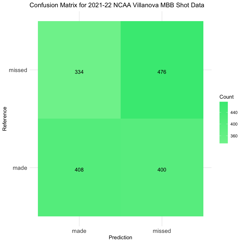
# Create a confusion matrixconf_matrix <- confusionMatrix(data = validation_predictions, reference = nova2122_validation$shot_outcome_numeric)# Print the confusion matrixprint(conf_matrix)
Confusion Matrix and Statistics

          Reference
Prediction  -1   1
        -1 476 400
        1  334 408

               Accuracy : 0.5464
                 95% CI : (0.5217, 0.5708)
    No Information Rate : 0.5006
    P-Value [Acc > NIR] : 0.0001276

                  Kappa : 0.0926

 Mcnemar's Test P-Value : 0.0164312

            Sensitivity : 0.5877
            Specificity : 0.5050
         Pos Pred Value : 0.5434
         Neg Pred Value : 0.5499
             Prevalence : 0.5006
         Detection Rate : 0.2942
   Detection Prevalence : 0.5414
      Balanced Accuracy : 0.5463

       'Positive' Class : -1
The accuracy of the above model, 0.5464, indicates that the model is accurate 54.64% of the time. The model has a precision of 0.5499, inicating that 54.99% of the model’s positive predictions are correct. The recall of the above model, 0.5877, indicates that the model correctly predicted 58.77% of the made shots. Finally, the F1-score (combines precision and recall of a classifier by taking their harmonic mean) of the model is 0.5681 which can be used to compare performance to other classifiers.
As evident in the initial matrix, the subsequent table, and the confusion matrix created using ggplot, the performance of the Naive Bayes model appears to be rather lackluster. With an accuracy rate slightly exceeding 50%, the model’s predictive ability seems only marginally better than random chance. This outcome aligns with the null hypothesis, indicating that the concept of a “hot hand” is likely a misconception, and past performance may not be a reliable predictor of success. It’s worth highlighting that applying Naive Bayes to time series data, as done here, may not be the most suitable approach, given the unique characteristics of this type of data.
Naive Bayes with Labeled Text Data
Switching back to Python, let’s perform Naive Bayes classification on the news data. Let’s take another look at the data.
Code
# what does the test data look like?
test_data.head()
Sentiment Label
cleaned_text
83
neutral
cbs sport network weekly coverage season keep ...
53
neutral
nfl week odds includes division matchup sunday...
70
neutral
removed
45
positive
real madrid look continue winning way keep per...
44
positive
florida gator hope end road game loss streak w...
We need to separate our features from our target variable which is done via the code below.
Code
# let's separate our feature(s) from our target variableX_test = test_data['cleaned_text']y_test = test_data['Sentiment Label']X_test.head()
83    cbs sport network weekly coverage season keep ...
53    nfl week odds includes division matchup sunday...
70                                              removed
45    real madrid look continue winning way keep per...
44    florida gator hope end road game loss streak w...
Name: cleaned_text, dtype: object
Since we know the feature column only includes the occurances of the word “win”, let’s create a new column ‘win_count’.
The following code chunk uses a Categorical Naive Bayes model from scikit-learn to predict the target variable (sentiment label) based on input features (win_count). It prepares the training and test datasets, handles missing values, fits the model, makes predictions, and evaluates the accuracy of the model on the validation set.
Code
import pandas as pdfrom sklearn.naive_bayes import CategoricalNBfrom sklearn.metrics import accuracy_score# Convert features to a DataFramenews_training_x = pd.Series(x_opt, name='x')news_training_y = y_trainnews_test_x = pd.Series(X_test_win, name='x')news_test_y = y_test# Create a training DataFrametraining_df = pd.DataFrame({'x': news_training_x, 'y': news_training_y})# Create a test DataFrametest_df = pd.DataFrame({'x': news_test_x, 'y': news_test_y})# Create a Naive Bayes modelnb_model = CategoricalNB()# Remove rows with NaN valuestraining_df.dropna(subset=['x'], inplace=True)test_df.dropna(subset=['x'], inplace=True)# Remove rows with NaN values in the target variable 'y'training_df.dropna(subset=['y'], inplace=True)test_df.dropna(subset=['y'], inplace=True)# Now, let's fit the modelnb_model.fit(training_df[['x']], training_df['y'])# Make predictions on the validation setvalidation_predictions = nb_model.predict(test_df[['x']])# and we can finally assess the accuracy of the modelaccuracy = accuracy_score(test_df['y'], validation_predictions)print("Accuracy of the Naive Bayes model:", accuracy)
Accuracy of the Naive Bayes model: 0.5
Code
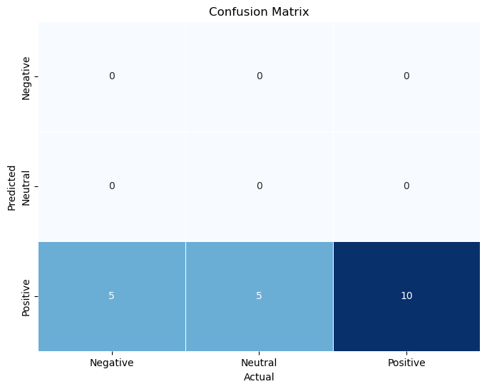
from sklearn.metrics import confusion_matrix# Create a confusion matrixconf_matrix = confusion_matrix(validation_predictions, test_df['y'])# Print the confusion matrixprint("Confusion Matrix:")print(conf_matrix)
Confusion Matrix:
[[ 0  0  0]
 [ 0  0  0]
 [ 5  5 10]]
Code
#calculate the various metricsaccuracy =10/20precision =10/20recall =10/10f1 =2* ((precision * recall) / (precision + recall))# Create a dictionary with the metricsmetrics = {'Metric': ['Accuracy', 'Precision', 'Recall', 'F1'],'Value': [accuracy, precision, recall, f1]}# Create a DataFrame from the dictionarymetrics_df = pd.DataFrame(metrics)print(metrics_df)
      Metric     Value
0   Accuracy  0.500000
1  Precision  0.500000
2     Recall  1.000000
3         F1  0.666667
The accuracy of the above model, 0.5, indicates that the model is accurate 50% of the time. The model has a precision of 0.5, inicating that 50% of the model’s positive predictions are correct. The recall of the above model, 1, indicates that the model correctly predicted 100% of the made shots. Finally, the F1-score (combines precision and recall of a classifier by taking their harmonic mean) of the model is 0.67 which can be used to compare performance to other classifiers.
Code
import seaborn as snsimport matplotlib.pyplot as plt# Assuming 'conf_matrix' is the confusion matrix obtained previously# Create a Seaborn heatmapplt.figure(figsize=(8, 6))sns.heatmap(conf_matrix, annot=True, fmt='d', cmap='Blues', linewidths=0.5, cbar=False, xticklabels=['Negative', 'Neutral', 'Positive'], yticklabels=['Negative', 'Neutral', 'Positive'])# Add labels and titleplt.xlabel('Actual')plt.ylabel('Predicted')plt.title('Confusion Matrix')# Show the heatmapplt.show()
Upon reviewing the initial matrix, subsequent table, and the Seaborn-generated confusion matrix, it becomes apparent that the Naive Bayes model’s performance is notably subpar. Despite achieving a 50% accuracy, a significant challenge emerges: the consistent prediction of positive label values points to a considerable underfitting problem. This result indicates that the employed Naive Bayes classifier was overly simplistic, resulting in inaccurate sentiment predictions for the news articles.
Extra Joke (x2)
Are monsters good at math? Not unless you Count Dracula.
What’s the official animal of Pi day? The Pi-thon!